from pylab import *
from scipy import *

# reading the data from a csv file
durl = 'http://datasets.flowingdata.com/crimeRatesByState2005.csv'
rdata = genfromtxt(durl,dtype='S8,f,f,f,f,f,f,f,i',delimiter=',')

rdata[0] = zeros(8) # cutting the label's titles
rdata[1] = zeros(8) # cutting the global statistics

x = []
y = []
color = []
area = []

for data in rdata:
 x.append(data[1]) # murder
 y.append(data[5]) # burglary
 color.append(data[6]) # larceny_theft
 area.append(sqrt(data[8])) # population
 # plotting the first eigth letters of the state's name
 text(data[1], data[5],
      data[0],size=11,horizontalalignment='center')

# making the scatter plot
sct = scatter(x, y, c=color, s=area, linewidths=2, edgecolor='w')
sct.set_alpha(0.75)

axis([0,11,200,1280])
xlabel('Murders per 100,000 population')
ylabel('Burglaries per 100,000 population')
show()
The following figure is the resulting bubble chart
It shows the number of burglaries versus the number of murders per 100,000 population. Every bubble is a state of America, the size of the bubbles represents the population of the state and the color is the number of larcenies.
Wednesday, November 23, 2011
How to make Bubble Charts with matplotlib
In this post we will see how to make a bubble chart using matplotlib. The snippet that we are going to see was inspired by a tutorial on flowingdata.com where R is used to make a bubble chart that represents some data extracted from a csv file about the crime rates of America by states. I used the dataset provided by flowingdata to create a similar chart with Python. Let's see the code:
Thursday, November 17, 2011
Fun with Epitrochoids
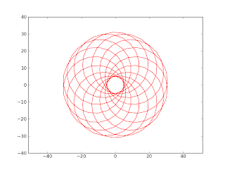
An epitrochoid is a curve traced by a point attached to a circle of radius r rolling around the outside of a fixed circle of radius R, where the point is a distance d from the center of the exterior circle [Ref]. Lately I found the Epitrochoid's parametric equations on wikipedia:
So,I decided to plot them with pylab. This is the script I made
So,I decided to plot them with pylab. This is the script I made
from numpy import sin,cos,linspace,pi
import pylab

# curve parameters
R = 14
r = 1
d = 18

t = linspace(0,2*pi,300)

# Epitrochoid parametric equations
x = (R-r)*cos(t)-d*cos( (R+r)*t / r )
y = (R-r)*sin(t)-d*sin( (R+r)*t / r )

pylab.plot(x,y,'r')
pylab.axis('equal')
pylab.show()
And this is the result
isn't it fashinating? :) Monday, November 7, 2011
Computing a disparity map in OpenCV
A disparity map contains information related to the distance of the objects of a scene from a viewpoint. In this example we will see how to compute a disparity map from a stereo pair and how to use the map to cut the objects far from the cameras.
The stereo pair is represented by two input images, these images are taken with two cameras separated by a distance and the disparity map is derived from the offset of the objects between them. There are various algorithm to compute a disparity map, the one implemented in OpenCV is the graph cut algorithm. To use it we have to call the function CreateStereoGCState() to initialize the data structure needed by the algorithm and use the function FindStereoCorrespondenceGC() to get the disparity map. Let's see the code:
Result using threshold = 100
The stereo pair is represented by two input images, these images are taken with two cameras separated by a distance and the disparity map is derived from the offset of the objects between them. There are various algorithm to compute a disparity map, the one implemented in OpenCV is the graph cut algorithm. To use it we have to call the function CreateStereoGCState() to initialize the data structure needed by the algorithm and use the function FindStereoCorrespondenceGC() to get the disparity map. Let's see the code:
def cut(disparity, image, threshold):
 for i in range(0, image.height):
  for j in range(0, image.width):
   # keep closer object
   if cv.GetReal2D(disparity,i,j) > threshold:
    cv.Set2D(disparity,i,j,cv.Get2D(image,i,j))

# loading the stereo pair
left  = cv.LoadImage('scene_l.bmp',cv.CV_LOAD_IMAGE_GRAYSCALE)
right = cv.LoadImage('scene_r.bmp',cv.CV_LOAD_IMAGE_GRAYSCALE)

disparity_left  = cv.CreateMat(left.height, left.width, cv.CV_16S)
disparity_right = cv.CreateMat(left.height, left.width, cv.CV_16S)

# data structure initialization
state = cv.CreateStereoGCState(16,2)
# running the graph-cut algorithm
cv.FindStereoCorrespondenceGC(left,right,
                          disparity_left,disparity_right,state)

disp_left_visual = cv.CreateMat(left.height, left.width, cv.CV_8U)
cv.ConvertScale( disparity_left, disp_left_visual, -16 );
cv.Save( "disparity.pgm", disp_left_visual ); # save the map

# cutting the object farthest of a threshold (120)
cut(disp_left_visual,left,120)

cv.NamedWindow('Disparity map', cv.CV_WINDOW_AUTOSIZE)
cv.ShowImage('Disparity map', disp_left_visual)
cv.WaitKey()
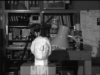
These are the two input image I used to test the program (respectively left and right):
Result using threshold = 100
Thursday, November 3, 2011
Face and eyes detection in OpenCV
The goal of object detection is to find an object of a pre-defined class in an image. In this post we will see how to use the Haar Classifier implemented in OpenCV in order to detect faces and eyes in a single image. We are going to use two trained classifiers stored in two XML files:
- haarcascade_frontalface_default.xml - that you can find in the directory /data/haarcascades/ of your OpenCV installation
- haarcascade_eye.xml - that you can download from this website.
imcolor = cv.LoadImage('detectionimg.jpg') # input image
# loading the classifiers
haarFace = cv.Load('haarcascade_frontalface_default.xml')
haarEyes = cv.Load('haarcascade_eye.xml')
# running the classifiers
storage = cv.CreateMemStorage()
detectedFace = cv.HaarDetectObjects(imcolor, haarFace, storage)
detectedEyes = cv.HaarDetectObjects(imcolor, haarEyes, storage)

# draw a green rectangle where the face is detected
if detectedFace:
 for face in detectedFace:
  cv.Rectangle(imcolor,(face[0][0],face[0][1]),
               (face[0][0]+face[0][2],face[0][1]+face[0][3]),
               cv.RGB(155, 255, 25),2)

# draw a purple rectangle where the eye is detected
if detectedEyes:
 for face in detectedEyes:
  cv.Rectangle(imcolor,(face[0][0],face[0][1]),
               (face[0][0]+face[0][2],face[0][1]+face[0][3]),
               cv.RGB(155, 55, 200),2)

cv.NamedWindow('Face Detection', cv.CV_WINDOW_AUTOSIZE)
cv.ShowImage('Face Detection', imcolor)
cv.WaitKey()
These images are produced running the script with two different inputs. The first one is obtained from an image that contains two faces and four eyes:
And the second one is obtained from an image that contains one face and two eyes (the shakira.jpg we used in the post about PCA):
Subscribe to:
Posts (Atom)


