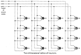
Notice: For an update tutorial on how to use minisom refere to the examples in the official documentation.The Self Organizing Maps (SOM), also known as Kohonen maps, are a type of Artificial Neural Networks able to convert complex, nonlinear statistical relationships between high-dimensional data items into simple geometric relationships on a low-dimensional display. In a SOM the neurons are organized in a bidimensional lattice and each neuron is fully connected to all the source nodes in the input layer. An illustration of the SOM by Haykin (1999) is the following
Each neuron n has a vector wn of weights associated. The process for training a SOM involves stepping through several training iteration until the item in your dataset are learnt by the SOM. For each pattern x one neuron n will "win" (which means that wn is the weights vector more similar to x) and this winning neuron will have its weights adjusted so that it will have a stronger response to the input the next time it sees it (which means that the distance between x and wn will be smaller). As different neurons win for different patterns, their ability to recognize that particular pattern will increase. The training algorithm can be summarized as follows:
- Initialize the weights of each neuron.
- Initialize t = 0
- Randomly pick an input x from the dataset
- Determine the winning neuron i as the neuron such that
- Adapt the weights of each neuron n according to the following rule
- Increment t by 1
- if t < tmax go to step 3
MiniSom is a minimalistic and Numpy based implementation of the SOM. I made it during the experiments for my thesis in order to have fully hackable SOM algorithm and lately I decided to release it on GitHub. The next part of this post will show how to train MiniSom on the Iris Dataset and how to visualize the result. The first step is to import and normalize the data:
from numpy import genfromtxt,array,linalg,zeros,apply_along_axis

# reading the iris dataset in the csv format
# (downloaded from http://aima.cs.berkeley.edu/data/iris.csv)
data = genfromtxt('iris.csv', delimiter=',',usecols=(0,1,2,3))
# normalization to unity of each pattern in the data
data = apply_along_axis(lambda x: x/linalg.norm(x),1,data)
The snippet above reads the dataset from a CSV and creates a matrix where each row corresponds to a pattern. In this case, we have that each pattern has 4 dimensions. (Note that only the first 4 columns of the file are used because the fifth column contains the labels). The training process can be started as follows:
from minisom import MiniSom
### Initialization and training ###
som = MiniSom(7,7,4,sigma=1.0,learning_rate=0.5)
som.random_weights_init(data)
print("Training...")
som.train_random(data,100) # training with 100 iterations
print("\n...ready!")
Now we have a 7-by-7 SOM trained on our dataset. MiniSom uses a Gaussian as neighborhood function and its initial spread is specified with the parameter sigma. While with the parameter learning_rate we can specify the initial learning rate. The training algorithm implemented decreases both parameters as training progresses. This allows rapid initial training of the neural network that is then "fine tuned" as training progresses.
To visualize the result of the training we can plot the average distance map of the weights on the map and the coordinates of the associated winning neuron for each patter:
from pylab import plot,axis,show,pcolor,colorbar,bone
bone()
pcolor(som.distance_map().T) # distance map as background
colorbar()
# loading the labels
target = genfromtxt('iris.csv',
                    delimiter=',',usecols=(4),dtype=str)
t = zeros(len(target),dtype=int)
t[target == 'setosa'] = 0
t[target == 'versicolor'] = 1
t[target == 'virginica'] = 2
# use different colors and markers for each label
markers = ['o','s','D']
colors = ['r','g','b']
for cnt,xx in enumerate(data):
 w = som.winner(xx) # getting the winner
 # palce a marker on the winning position for the sample xx
 plot(w[0]+.5,w[1]+.5,markers[t[cnt]],markerfacecolor='None',
   markeredgecolor=colors[t[cnt]],markersize=12,markeredgewidth=2)
axis([0,som.weights.shape[0],0,som.weights.shape[1]])
show() # show the figure
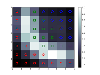
The result should be like the following:
For each pattern in the dataset the corresponding winning neuron have been marked. Each type of marker represents a class of the iris data ( the classes are setosa, versicolor and virginica and they are respectively represented with red, green and blue colors). The average distance map of the weights is used as background (the values are showed in the colorbar on the right). As expected from previous studies on this dataset, the patterns are grouped according to the class they belong and a small fraction of Iris virginica is mixed with Iris versicolor.
For a more detailed explanation of the SOM algorithm you can look at its inventor's paper.


